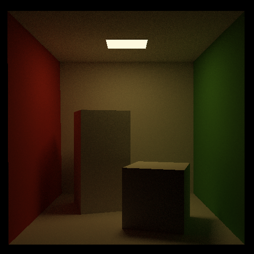
Path tracing is a physically based rendering technique that simulates the complex ways light interacts with surfaces to produce realistic images. It builds on the principles of ray tracing but extends them to capture global illumination, including indirect lighting, color bleeding, reflections, and refractions. By following rays of light as they bounce through a scene and averaging the results of many random samples, path tracing can closely approximate the real-world physics of light transport, producing images with a high degree of realism at the cost of greater computational effort.
The full implementation is maintained in a private repository. I’m happy to provide code excerpts or discuss the architecture upon request.
Rendering Equation
At the heart of path tracing is Kajiya’s rendering equation, which describes the amount of light leaving a point in a given direction:
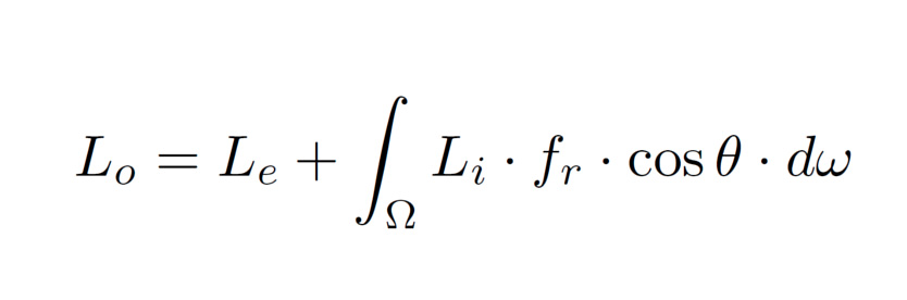
The equation calculates the amount of outgoing light in a particular direction from a particular point (Lo) as the sum of the light being emitted from point (Le) and the amount of incoming light being reflected in that particular direction (the integral expression). The integral expression sums up the contributions of light arriving from every possible incoming direction above the surface, and weights them by how the surface reflects (fr cosθ) and how much of that light actually hits the surface (Li).
BRDFs
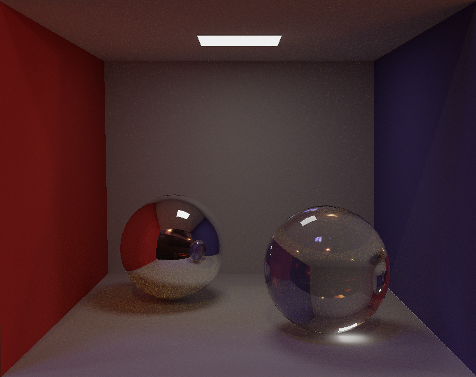
The term fr in the rendering equation — the bidirectional reflectance distribution function (BRDF) — describes how light arriving from one direction is reflected toward another. In essence, the BRDF encodes a material’s reflective properties. By choosing different BRDF models, we can simulate a wide variety of materials in a physically based way.
My path tracer currently implements the following BRDFs:
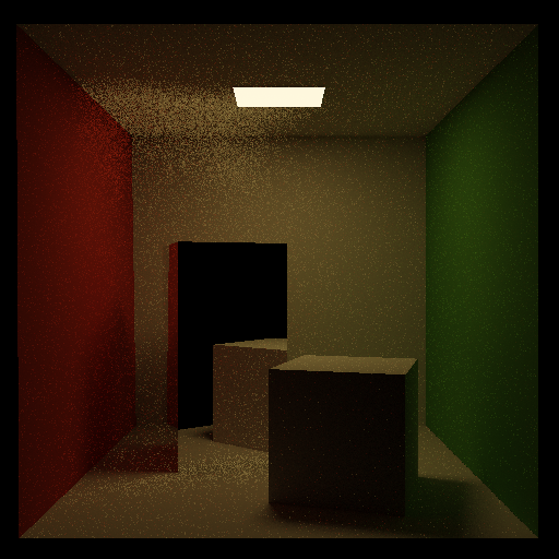
- Lambertian diffuse: light is scattered equally in all directions, producing a matte appearance.
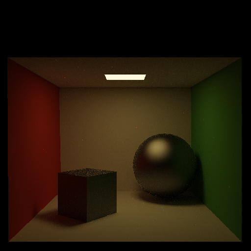
- Glossy specular: light reflection is concentrated around the mirror direction, controlled by surface roughness.
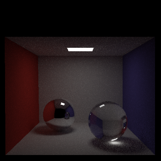
- Perfect mirror: light is reflected only in the exact mirror direction, with no scattering.
- Fresnel dielectric refraction: light can be reflected or refracted through the surface depending on the incident angle, as governed by the Fresnel equations.
- Cook–Torrance microfacet: models a surface as a collection of tiny mirror-like facets, capturing rough, physically plausible highlights.
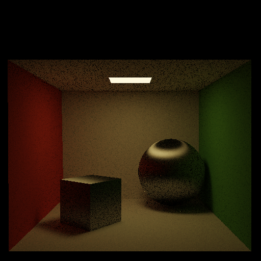
- Ward anisotropic: extends microfacet theory to handle direction-dependent roughness, producing stretched highlights for materials like brushed metal.
Implementation
Like in ray tracing, a ray is cast in the direction of each pixel, with the amount of incoming light determining the pixel’s color. The rendering equation is treated as a function that is recursively called: the incoming light at a point depends on light leaving other points, which themselves depend on light arriving from yet more points, and so on. When you follow this chain, you see that a single camera ray can spawn a sequence of “bounces” as it reflects, refracts, or scatters around the scene before eventually hitting a light source or leaving the scene entirely.
However, in path tracing, we can’t compute the rendering equation exactly: the integral over all incoming directions is far too complex. But, even if we numerically integrate over all possible incoming directions, the recursion means that rendering time will very quickly blow out of proportion.
That’s where Monte Carlo integration comes in. Instead of evaluating the integral over every possible incoming direction at each bounce, we randomly pick one or more directions to sample and recursively trace them. We repeat this process for many samples, sum their contributions, and divide by the number of samples, giving us an unbiased estimate of the true integral.
To prevent rays from bouncing indefinitely, we use a technique called Russian roulette. After a certain number of bounces, each path is given a survival probability based on its current contribution (throughput). With that probability, we either continue tracing the path or terminate it early. If the path survives, its contribution is scaled by the inverse of the survival probability to keep the estimate unbiased. This way, we save computation on low-energy paths without darkening the image.
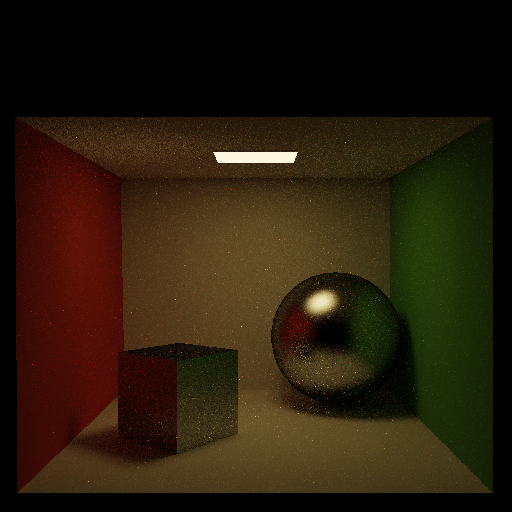
The trade-off is noise: fewer samples per pixel mean grainier images, but as more samples are taken, the result converges toward the physically correct solution.
Because the path tracer works in high dynamic range (HDR), pixel values can vary over many orders of magnitude, far beyond what a standard display can show. Without tone mapping, bright areas would clip to pure white and dark areas would lose detail. So, the path tracer uses the extended Reinhard operator to compress this wide range into the displayable range while preserving contrast and detail.
A lot of the noise from Monte Carlo rendering is a result of the fact that random samples may cluster unevenly, leaving gaps in coverage. Low-discrepancy sequences (also called quasi-random sequences) are designed to spread samples more evenly across the domain. In my path tracer, low-discrepancy sampling is used for both pixel sampling and directional sampling on the hemisphere, producing cleaner images at lower sample counts.
Additional Features
In addition to core global illumination, the path tracer supports a few features that enhance realism and artistic control:
- Depth of Field: Implemented using a thin-lens camera model. For each sample, the camera ray’s origin is randomly jittered over a virtual aperture, and its direction adjusted so it focuses at a chosen focal distance. This mimics real camera optics, producing natural blur for objects in front of or behind the focal plane.
- HDRI Environment Lighting: The renderer can use a high-dynamic-range image (HDRI) as a background and light source. Rays that miss scene geometry sample the HDRI in their outgoing direction, both displaying the image and contributing realistic, image-based lighting with soft shadows and natural color tones.


